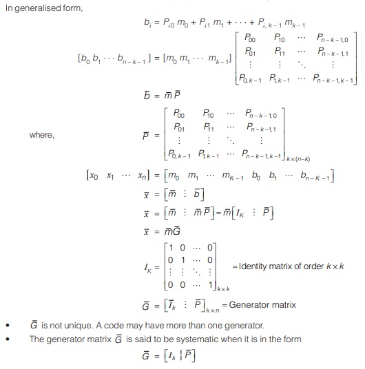
Additive White Gaussian Noise Channel (AWGN)

If the channel is affected by White Noise then it is called as AWGN channel. White Noise is basically thermal noise.
In an additive white Gaussian noise channel, the channel output y is given by

y = x + n

where, x is channel input and n is an additive band limited white Gaussian noise with zero mean and variance σ².

Capacity C_s of an AWGN channel is given by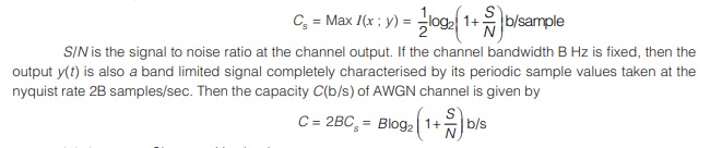

It is known as Shannon Hartley law.
Hence, it is easier to increase the information capacity of a continuous communication channel by expanding its bandwidth than by increasing the transmitted power for a prescribed noise variance.

Source Coding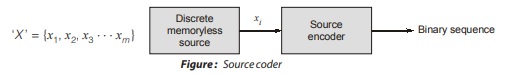

A conversion of the output of a discrete memoryless source into a sequence of symbols (i.e. binary code word) is called source coding.
Objective: An Objective: objective of source coding is to minimize the average bit rate to achieve the efficient representation of data generated by source by removing redundancy.

Important Terms

Let ‘X ’ be a DMS with finite entropy H(X) and an alphabet {x₁, x₂ ⋅ ⋅ ⋅ x_m} with corresponding probabilities of occurrence P(x_i) (i = 1, 2 ⋅ ⋅ ⋅ m). Let the binary code word assigned to symbol x_i by the encoder have length n_i , measured in bits. The length of a codeword length of a codeword is the number of binary digits in the codeword. The average code word code word length L, per source symbol is given by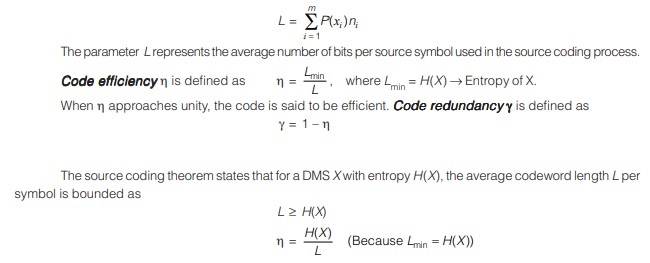

Error Control Coding

When a signal is transmitted through channel, the probability of error for a particular signalling scheme is function of signal to noise ratio at receiver input and information rate. In practical systems, maximum signal power, the bandwidth of channel and noise power spectral density No/2 are fixed for particular environment.
Using signalling scheme, it is not possible often to achieve acceptable probability of error. Therefore, error control coding is used to achieve required minimum probability of error.
Methods of error correction are:

ARQ	FEC
· ARQ stands for Automatic Repeat request · When an error is detected, a request is sent to transmitter from receiver to retransmit the signal. · It needs duplex arrangement. · Time delays are involved due to request and repeat signals, therefore it cannot be used in real time signals.	· FEC stands for forward error correction. · In automatic mechanism of error correction in the form of error correction code is employed and hence no retransmission occurs · It needs simplex arrangement. · No delays are involved. Hence, it can be used in real time signals.

Parity Check Code

The parity check is done by adding an extra bit, called parity bit, to the data to make the number of 1s either even or odd depending upon the type of parity. The parity check is suitable for single bit error detection only.

When the number of check bits is one, it is known as parity check code. It is of two types:

• Even Parity Check Code
  If check bit is such that total number of 1’s in the code word is even, it is even parity check code.
• Odd Parity Check Code
  When the check bit is such that total number of 1’s in code word is odd, it is called odd parity check code.

Message	Code for even parity Check bit	Code for odd parity Check bit
010011	1	0
101110	0	1

If single error occurs in received message, it can be easily detected as it changes the number of 1’s from even to odd or from odd to even.

Important Definitions

Code word

• It is the block of bits at the output of channel encoder

Code rate

r = Number of bits in message block/ Number of bits in encoded codeword = k/n ≤ 1

R_b = Bit rate before channel encoding = 1/T_b

R_o = Bit rate (or channel data rate) after channel encoding = 1/T_o

kT_b = nT_o

Code Efficiency

Code efficiency = k/n = Code rate

Hamming Weight of a Code word W(x)

W(x) = Number of non zero elements in the given code word.
eg: Hamming weight of a binary code word “11010001” is “4”.

Hamming Distance
The Hamming distance, between two code words, is the number of locations in which their respective
elements differ.
e.g.: Hamming distance between the code words “1011010” and “0111000” is 3

Hamming Distance

The Hamming distance, between two code words, is the number of locations in which their respective
elements differ.
e.g.: Hamming distance between the code words “1011010” and “0111000” is 3At these three locations bits in two given code words are different. So the Hamming distance between the two given code words is “3”

Hamming distance between two given code words also can be defined as the Hamming weight of the code word obtained by the addition (Exclusive-OR) of the given two code words. weight of the code word obtained by the addition (Exclusive-OR) of the given two code words.
e.g.: Hamming distance between the code words “1011010” and “0111000” is given by,
(1011010) ⊕ (0111000) = (1100010)

Some properties of Hamming distance between two code words
d(x, y) = Hamming distance between the code words x and y. Then

d(x, y) ≥ 0 → with equality if x = y
d(x, y) = d(y, x) → Symmetry
d(x, y) ≤ d(x, z) + d(z, y) → Triangle inequality

Minimum Distance (d_min)

• It is the smallest value of the Hamming distance between any pair of code words in the given coding system.
• It is also can be defined as the smallest Hamming weight of non zero code words in the coding system. (if all zeros is a code word in that coding system. e.g.: linear block codes)

Relation between d_min and detection and correction capabilities of the code:

Capability	Condition
Detect upto “s ” errors per word.	dmin ≥ (s + 1)
Detect and Correct upto “t ” errors per word.	dmin ≥ (2t + 1)
Correct upto “t ” errors and Detect “s ≥ t ” errors per word.	dmin ≥ (t + s + 1)

Linear Code

A code is said to be linear when the addition (Modulo-2) of two different code words produces another valid code word in the same coding system.

Linear Block Codes

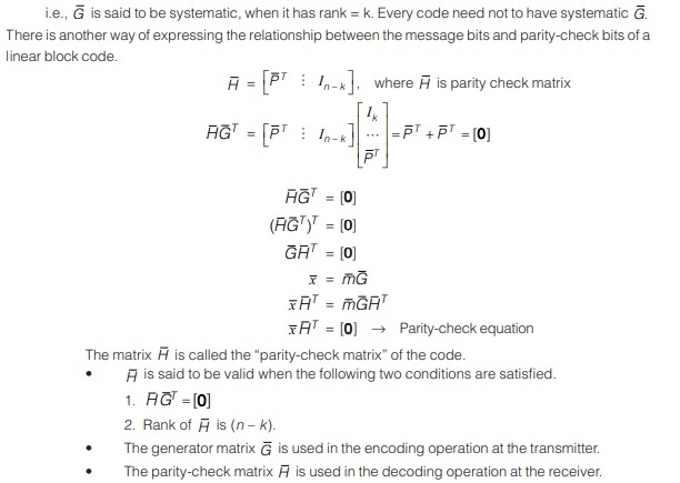
Properties of Linear Block Codes (LBCs)

An LBC remains unchanged if the generator matrix is subjected to elementary row operation. Suppose you can form a new code by choosing any two components and transposing the symbols in these two components. This gives a new code which will be also an LBC.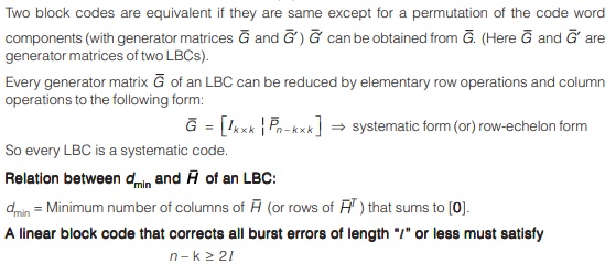

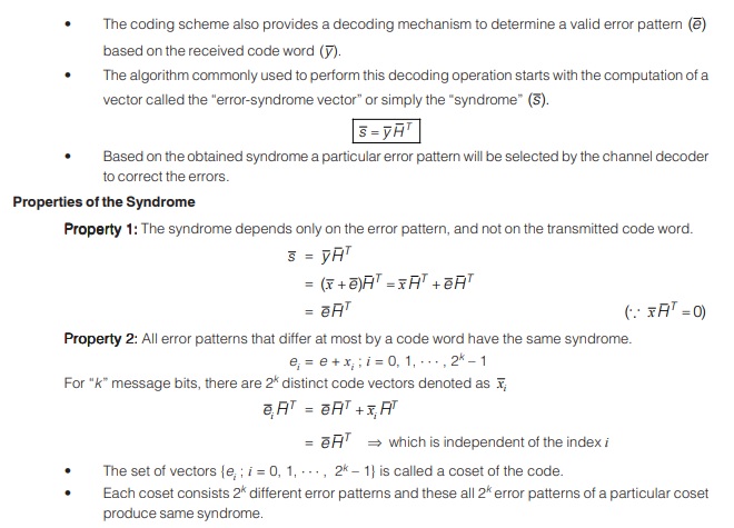
Syndrome Decoding

When the encoded code word is transmitted through a noisy channel, some error will occur in the received code word. Let this error code word is denoted by “ y ”.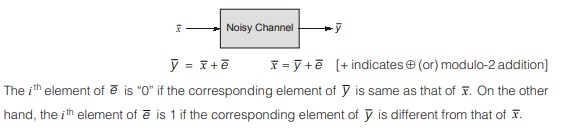

Cyclic Redundancy Checks (CRC)

This Cyclic Redundancy Check is the most powerful and easy to implement technique which is based on binary division. The procedure can be explained in the following steps :

1. A sequence of redundant bits, called cyclic redundancy check bits, are appended to the end of data unit.
2. The resulting data unit becomes exactly divisible by a second, predetermined binary number.
3. At the destination, the incoming data unit is divided by the same number.
4. If at this step there is no remainder, the data unit is assumed to be correct and is therefore accepted.
5. Remainder indicates that the data unit has been damaged in transit and therefore must be rejected.

Assume if a k bit message is to be transmitted, the transmitter generates an r-bit sequence, known as Frame Check Sequence (FCS) so that the (k + r) bits are actually being transmitted. Now this r-bit FCS is generated by dividing the original number, appended by r zeros, by a predetermined number. This number, which is (r + 1) bit in length, can also be considered as the coefficients of a polynomial, called Generator Polynomial. The remainder of this division process generates the r-bit FCS. On receiving the packet, the receiver divides the (k + r) bit frame by the same predetermined number and if it produces no remainder, it can be assumed that no error has occurred during the transmission. Operations at both the sender and receiver end as shown in the figure below.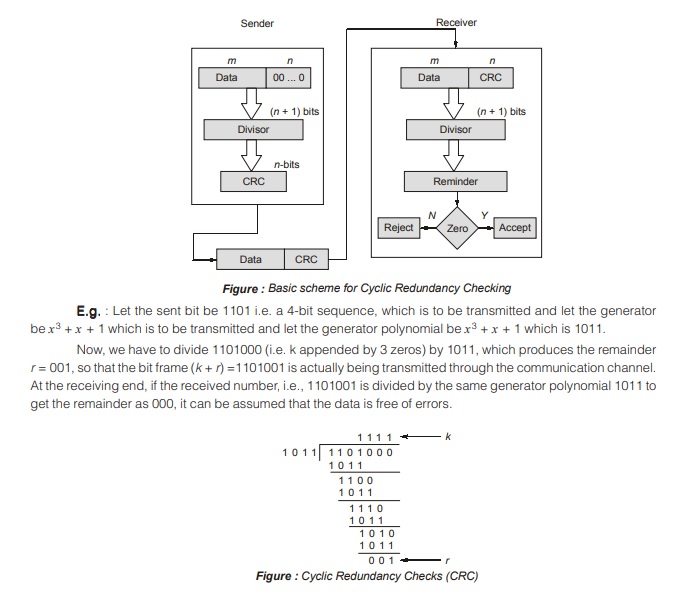

The transmitter can generate the CRC by using a feedback shift register circuit and the same circuit can also be used at the receiving end to check whether any error has occurred. All the values can be expressed as polynomials of a dummy variable X. The polynomial is selected to have at least the following properties :

1. It should not be divisible by X. This condition guarantees that all burst errors of a length equal to the degree of polynomial are detected.
2. It should not be divisible by (X + 1). This condition guarantees that all burst errors affecting an odd number of bits are detected.
   CRC process can be expressed as XⁿM(X)/P(X) = Q(X) + R(X) / P(X)

Performance

CRC is a very effective error detection technique. If the divisor is chosen according to the previously mentioned rules, its performance can be summarized as follows:

• CRC can detect all single-bit errors 1.
• CRC can detect all double-bit errors (three 1’s) 2.
• CRC can detect any odd number of errors ( 3. X + 1)
• CRC can detect all burst errors of less than the degree of the polynomial. 4.
• CRC detects most of the larger burst errors with a high probability.

Error Correcting Codes

The techniques that we have discussed so far can detect errors, but do not correct them. Error Correction can be handled in two ways.

Backward error correction : It is when an error is discovered; the receiver can have the sender retransmit the entire data unit.
Forward error correction : In this the receiver can use an error-correcting code, which automatically corrects certain errors.

In theory it is possible to correct any number of errors atomically. Error-correcting codes are more sophisticated than error detecting codes and require more redundant bits. The number of bits required to correct multiple-bit or burst error is so high that in most of the cases it is inefficient to do so. For this reason, most error correction is limited to one, two or at the most three-bit errors.