Digital Filters

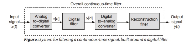
A digital filter uses computation to implement the filtering action that is to be performed on a continuous time signal. Figure shows a block diagram of the operations involved in such an approach to design a frequency selective filter. The block labeled “Analog-to-digital (A/D) converter” is used to convert the continuous-time signal x(t) into a corresponding sequence x[n] of numbers. The digital filter processes the sequence of numbers x[n] on a sample-by-sample basis to produce a new sequence of number, y[n], which is then converted into the corresponding continuous-time signal by the digital-to-analog (D/A) converter. Finally, the reconstruction (low pass) filter at the output of the system produces a continuous-time signal y(t), representing the filtered version of the original input signal x(t).

Two important points should be carefully noted in the study of digital filters:

1. The underlying design procedures are usually based on the use of an analog or infinite precision model for the samples of input data and all internal calculations; this is done in order to take advantage of well-understood discrete-time, but continuous-amplitude. The resulting discrete-time filter provides the designer with a theoretical framework for the task at hand.
2. When the discrete-time filter is implemented in digital form for practical use, as depicted in figure below, the input data and internal calculations are all quantized to a finite precision. In doing so, round-off errors are introduced into the operation of the digital filter, causing its performance to deviate from that of the theoretical discrete time filter from which it is derived.

In this section, we confine ourselves to matters, relating to point 1. Although, in light of this point, the filters considered herein should in reality be referred to as discrete-time filters, we will refer to them as digital filters to conform to commonly used terminology.

Analog filters are characterized by an impulse response of infinite duration. In contrast, there are two classes of digital filters, depending on the duration of the impulse response:

Finite-duration impulse response (FIR) digital filters, the operation of which is governed by linear constant coefficient difference equations of a non-recursive nature. The transfer function of an FIR digital filter is a polynomial in z^–1. Consequently, FIR digital filters exhibit three important properties:

• They have finite length impulse response.
• They are always BIBO stable.
• They can realize a desired magnitude response with an exactly linear phase response (i.e., with no phase distortion).

Infinite-duration impulse response (IIR) digital filters, whose input-output characteristics are governed by linear constant-coefficient difference equations of a recursive nature. The transfer function of an IIR digital filter is a rational function in z^–1. Consequently, for a prescribed frequency response, the use of an IIR digital filter results in simple and less costly circuitry than does the use of the corresponding FIR digital filter. However, this improvement is achieved at the expense of phase distortion and a transient start-up that is not limited to a finite time interval.

Basics Structures for IIR Systems

Causal IIR systems are characterized by the constant coefficient difference equation or equivalently, by the real rational transfer function of equation. From these equations, it can be seen that the realization of infinite duration impulse response (IIR) systems involves a recursive computational algorithm. In this section, the most important filter structures namely direct Forms-I and II, cascade and parallel realizations for IIR systems are discussed.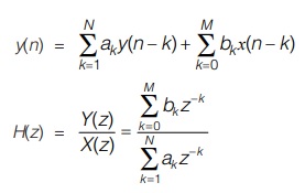

Basic Structures for FIR Systems

The system function of the FIR system whose realization take the form of a non-recursive computational algorithm may be written as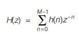

That is, if the impulse response is M samples in duration, the H(z) is a polynomial in z^–1 of degree M – 1. Thus H(z) has (M – 1) poles at z = 0 and (M – 1) zeros that can be anywhere in the finite z-plane.

FIR filters are often preferred in many applications, since they provide an exact linear phase over the whole frequency range and they are always BIBO stable independent of the filter coefficients. Two simple realization methods for FIR filters, viz. direct form and cascade form are outlined below.

Direct Form Realization of FIR System

The convolution sum relationship gives the system response as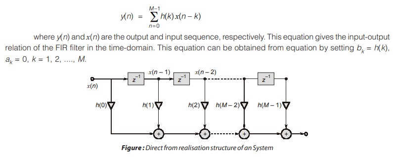

The direct form realization for equation in shown in above figure. This is similar to that of figure when all the coefficients a_k = 0. Hence, the direct form realization structure for FIR system is the special case of the direct form realization structure for IIR system.
The transposed structure shown in figure below is the second direct form structure. Both of these direct form  structures are canonic with respect to delays.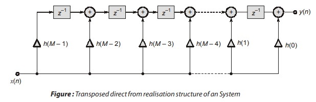

Comparison between FIR and IIR Filter