Conditional Probability

It often happens that the probability of one event is influenced by the outcome another event. As an example, consider drawing two cards in succession from a deck. Let A denote the event that the first card drawn is an ace. We do not replace the card drawn in the first trial. Let B denote the event that the second card drawn is an ace. It is evident that the probability of drawing an ace in the second trial will be influenced by the outcome of the first draw. If the draw does not result in an ace, then the probability of obtaining an ace in the second trial is 4/51.

The probability of event B thus depends on whether event A occurs.
Conditional probability P(B|A) denote the probability of event B when it is known that event A has occurred. P(B|A) is read as “probability of B given A”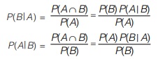This relation is known as Baye’s rule.
In Baye’s rule, one conditional probability is expressed in terms of the reversed conditional probability.

Random Variable

The outcome of an experiment may be a real number or it may be non-numerical and describable by a phrase (such as “heads” or “tail” in tossing a coin).
From a mathematical point of view, it is simpler to have numerical value for all outcomes. For this reason, we assign a real number to each sample point according to some rule.

The probability of an RV “X” taking a value x_i is

Px(x_i) = Probability of “X” = x_i

Conditions for Function to be a Random Variable

Thus, a random variable may be almost any function we wish. We shall, however, require that it not be multivalued. That is, every point in sample space ‘S’ must correspond to only one value of the random variable. Moreover, we shall require that two additional conditions be satisfied in order that a function X be a random variable. First, the set {X ≤ x} shall be an event for any real number x. The satisfaction of this condition will be no trouble in practical problems. This set corresponds to those points s in the sample space for which the  random variable X(s) does not exceed the number x. The probability of this event, denoted by P(X ≤ x), is equal to the sum of the probabilities of all the elementary events corresponding to {X ≤ x}.

The second condition we require is that the probabilities of the events {X = ∞} and {X = –∞} be 0.

P{X = –∞}=0
P{X = ∞}=0

This condition does not prevent X from being either –∞ or ∞ for some values of S; it only requires that the probability of the set of those s be zero.

Discrete and Continuous Random Variables

A discrete random variable is one having only discrete values. The sample space for a discrete random variable can be discrete, continuous, or even a mixture of discrete and continuous points. For example, the “wheel of chance when spun, the possible outcomes are the numbers from 0 to 12 marked on the wheel,” has a continuous sample space, but we could define a discrete random variable as having the value 1 for the set of outcomes {0 < s ≤ 6} and –1 for {6 < s ≤ 12}. The result is a discrete random variable defined on a continuous sample space.
A continuous random variable is one having a continuous range of values. It cannot be produced from a discrete sample space because of our requirement that all random variables be single-valued functions of all sample-space points. Similarly, a purely continuous random variable cannot result from a mixed sample space because of the presence of the discrete portion of the sample space.

Mixed Random Variable

A mixed random variable is one for which some of its values are discrete and some are continuous. The mixed case is usually the least important type of random variable, but it occurs in some problems of practical significance.

Distribution Function CDF Specifies the Probability of a RV ‘X ’ Taking Values upto ‘X’

The probability P {X ≤ x} is the probability of the event{X ≤ x}. It is a number that depends on x; that is, it is a function of x. We call this function, denoted F_X(x), the cumulative probability distribution function of the random variable X. Thus,

F_X(x) = P {X ≤ x}

We shall often call F_X(x) just the distribution function of X. The argument x is any real number ranging from –∞ to ∞. The distribution function has some specific properties derived from the fact that F_X(x) is a probability.
These are: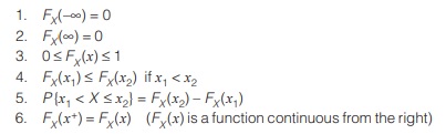

Stochastic Processes or Random Processes

A random process is a natural extension of the concept of random variable when dealing with signal. In analyzing communication systems we are basically dealing with time varying signals. In our development so far, we have assumed that all the signals are deterministic. In many situations the deterministic assumption on time varying signals is not a valid assumption, and it is more appropriate to model signals as random rather than deterministic function. One such example is the case of thermal noise in electronic circuits. This type of noise is due to the random movement of electrons as a result of thermal agitation and therefore, the resulting current and voltage can only be described statistically.
Another example is the reflection of radio waves from different layers of the ionosphere that makes long rang broadcasting of short-wave radio possible. Due to randomness of this reflection, the received signal can again be modeled as a random signal. These two examples show that random signals are suitable for description of certain phenomena in signal transmission.

Another situation where modeling by random processes proves useful is in the characterization of information source. An information source, such as a speed source, generates time varying signals whose contents are not known in advance, otherwise there would be no need to transmit them. Therefore, random process provide a natural way to model information sources as well.
The way to think about the relationship between probability theory and stochastic processes is as follows. When we consider the statistical characterization of a stochastic process at a particular instant of time, we are basically dealing with the characterization of a random variable sampled (i.e. observed) at that instant of time. When, however, we consider a single realization of the process, we have a random waveform that evolves across time. The study of stochastic processes, therefore, embodies two approaches: one based on ensemble averaging and the other based on temporal averaging. Both approaches and their characterizations are considered in this chapter.
Stochastic processes have two properties. First, they are functions of time. Second, they are random in the sense that, before conducting an experiment, it is not possible to define the waveforms that will be observed in the future exactly.

Consider, then, a stochastic process specified by
(a) Outcomes s observed from some sample space S,
(b) Events defined on the sample space S and
(c) Probabilities of these events.
Suppose that we assign to each sample point s a function of time in accordance with the rule

X(t, s), –T ≤ t ≤ T

Where 2T is the total observation interval. For a fixed sample point sj, the graph of the function X(t, sj) versus time t is called a realization or sample function of the stochastic process. To simplify the notation,

we denote this sample function as

x_j (t) = X(t, sj)

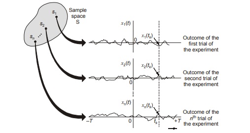
A stochastic process X(t) is an ensemble of time function, which together with a probability rule, assigns a probability to any meaningful event associated with an observation of one of the sample functions of the stochastic process.

Mean, Correlation, and Covariance Functions of Weakly Stationary Processes

Consider a real-valued stochastic process X(t). We define the mean of the process X(t) as the expectation of the random variable obtained by sampling the process at some time t, as shown by

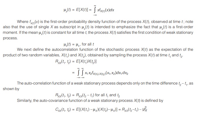
Properties of the Autocorrelation Function

Property 1: Mean-square value

The mean-square value of a stationary process X(t) is obtained from autocorrelation function R_XX(τ) simply by putting τ = 0 as shown by

R_XX(0) = E[X²(t)] = Mean square value = Total power

Property 2 : Symmetry

The auto-correlation function R_XX(τ) is an even function of the time shift τ ; that is,

R_XX(τ) = R_XX(– τ)

It is an even function.

Property 3 : Bound on the autocorrelation function

The autocorrelation function RXX(τ) attains its maximum magnitude at τ = 0; that is,

|R_XX(τ)| ≤ R_XX(0)

Property 4: normalization

Values of the normalized autocorrelation function

ρ_XX(τ) = R_XX(τ)/R_XX(0)

are confined to the range [–1, 1].