Traffic Studies and Analysis
Traffic studies or surveys are carried out to analyze the traffic characteristics. A detailed knowledge of the operating characteristics of the traffic is essential to form a basis for the establishment of traffic control or for design of highways.
The results of data collected are used in
(i) Traffic planning
(ii) Traffic management
(iii) Economic studies
(iv) Traffic and environmental control
(v) Monitoring trends
Traffic studies are broadly classified into two categories:
(i) Those concerned with the characteristics of traffic in transit
(a) Traffic volume study
(b) Speed studies
(c) Origin and destination study
(d) Traffic flow characteristics and studies
(e) Traffic capacity studies
(ii) Those related to land use movements
(a) Parking Studies
(b) Accident Studies
TRAFFIC FLOW CHARACTERISTICS AND STUDIES
A traffic stream is generally characterized by three key parameters:
(i) Speed of Stream
The speed of a traffic stream is defined as the average speed of all the vehicles over a period of time. Averaging of speed of vehicles can be done in two ways i.e. Arithmetic mean and harmonic mean known as time mean speed and space mean speed respectively.
However, space mean speed is preferred over time mean speed because space mean speed gives better description of stream conditions as it give a measure of speed of traffic stream over space. It is usually expressed as kmph.
(ii) Traffic Density, k
It is defined as average number of vehicle occupying a unit distance of a road at a given instant. It is simply determined by dividing the total number of vehicles occupying a length of road section by that length of road section at a instant of time. Hence, the unit of density, k is generally taken as vehicles per km.
(iii) Traffic Flow or Volume, q
As already discussed, traffic flow or traffic volume can be defined as total number of vehicles of stream that crossed a fixed point on the road over a unit period of time. It is usually expressed as vehicle per unit time (vph).
Macroscopic Traffic flow Models
Studies on traffic flow pattern has shown that there is inter-relationship among k and u also apart from the fundamental relation of traffic flow.
It can be said that all the 3 key parameters i.e. speed, density and volume are related to each other pairwise. There is a relationship between
(i) Speed and density
(ii) Density and volume
(iii) Volume and speed
However, relationship between speed and density can be thought off as most basic among the 3 relationships. The reason for assuming it as most basic is its application in practical situations. A driver driving his car on a road reduce or increases the speed according to the vehicles surrounding him. If the density of traffic stream surrounding the driver of vehicle is high, then the driver would have to reduce his speed and vice-versa.
Hence, as the relation between density of traffic stream and speed of traffic stream is an outcome of behavioural aspect of driver so, it is the basic relation.
Now, various traffic models has been proposed over the years which relates speed and density and other relations are derived using fundamental equation of traffic flow in these models.
Before studying these models, some important terms are required which are as follows:
(i) Free-flow speed, Usf: The speed of traffic stream when the density of traffic stream is very low is known as free flow speed.
(ii) Jam density kj : The density of stream when speed of stream reaches its lower limit i.e. nearly equal to zero is known as jam density.
Among many models describing relation between speed and density, some of the models are as follows:
1. Linear model
2. Logarithmic model
3. Exponential model
4. Generalised polynmial model
5. Multi-regime model
(a) Linear Model
It was proposed by Greenshield. As per his model, speed of stream is a linear function of density described by the equation:
u = a + bk …(i)
where, u = speed of stream
k = density of stream
a and b are constants which can be evaluated using boundary condition as:
At u = 0, k = kj …(ii) (∵ As discussed earlier)
u = usf, k = 0 …(iii) (∵ As discussed earlier)
Putting (ii) and (iii) in (i), we get
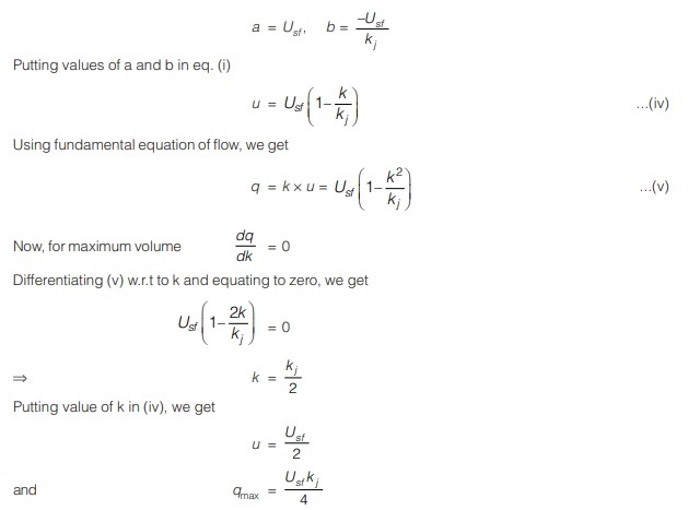
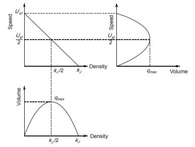
The relationship among 3 parameters using greenshield’s model is shown in the figure below.
<< Previous | Next >>
Must Read: What is Highway Engineering?
Dear Aspirants,
Your preparation for GATE, ESE, PSUs, and AE/JE is now smarter than ever — thanks to the MADE EASY YouTube channel.
This is not just a channel, but a complete strategy for success, where you get toppers strategies, PYQ–GTQ discussions, current affairs updates, and important job-related information, all delivered by the country’s best teachers and industry experts.
If you also want to stay one step ahead in the race to success, subscribe to MADE EASY on YouTube and stay connected with us on social media.
MADE EASY — where preparation happens with confidence.
MADE EASY is a well-organized institute, complete in all aspects, and provides quality guidance for both written and personality tests. MADE EASY has produced top-ranked students in ESE, GATE, and various public sector exams. The publishing team regularly writes exam-related blogs based on conversations with the faculty, helping students prepare effectively for their exams.