Shock Waves

Whenever a stream of traffic flowing under some flow condition (say, speed = u_A, density = k_A and flow = q_A) meets another stream of traffic flowing under some other conditions (say, speed = u_B, density = k_b and flow = q_b), then a wave is assumed to be generated known as shock wave. To shock wave have better understanding of shock waves, consider a single lane road on which few vehicles are moving in a line. Assume that all the vehicles have same speed while moving on the road so that the distance between the vehicles will remain constant. The speed with which vehicles are moving can be termed as speed of traffic stream. For instance, let the speed of stream is 80 kmph. Now, at an intersection, a truck comes on the road having a speed of 20 kmph.

A platoon is generally defined as a group of vehicles travelling together, either voluntarily or involuntarily, because of signal control, geometric or other factors. It can be said that a shock wave is generated which has decreased the speed of vehicles behind the truck. Now, let after some time, truck has moved out of road through an intersection. Now, the vehicles will start to accelerate. Again, it can be said that a shock wave is generated which has increased the speed of platoon.

Speed of Shock wave

Let a stream condition having characteristics u_A, k_A, q_A meets another stream condition having characteristics u_B, k_B, q_B. As the two flow conditions are meeting, therefore a shock wave should be generated. So, speed of shock wave, usw can be obtained as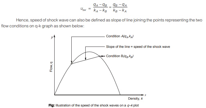

As per speed criteria, shock wave can be divided into three types:

1. The forward moving shock wave, i.e. the shock wave having positive speed represented by line-1 in the figure below.
2. The stationary shock wave i.e. the speed of shock wave is zero, represented by line-2 in the figure below.
3. The backward moving shock wave, i.e. the speed of shock wave is negative represent by line -3 in the figure below.

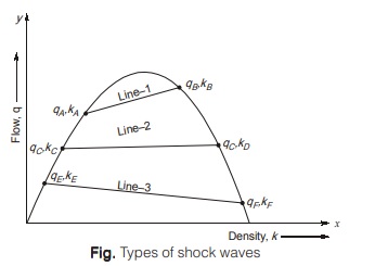
As it is clear from the figure that

1. A forward moving shock wave represented by line-1 is formed when a stream with lower flow and lower density meets and stream with higher flow and higher density or when a stream with higher density and higher flow meets a stream with lower flow and lower density.
2. A stationary shock wave will occur when the streams meets having same flow but different densities.
3. A backward moving shock wave is formed when a stream having higher flow and lower density meets a stream having lower flow and higher density or when a stream having lower flow and higher density meets a stream with higher flow and lower density.

DELAY AND QUEUE ANALYSIS

In this analysis, delay faced by vehicles at signalized intersection and queues developed at signalized intersection is studied with the help of number of vehicles arriving and departing at intersection. To start with, a plot is drawn in which time is taken on x-axis and on y-axis, cumulative number of vehicle that arrive and depart at the intersection are taken and curve is plotted based on data.

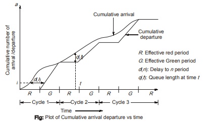
In the figure, the time on x-axis is divided in time of cycles. Each cycle is divided into two parts.

• R represent effective red time in which there is no departure of vehicle. Consequently, the slope of cumulative departure curve in the ‘R’ portion is zero or it can be said that number of vehicles departing from intersection in that time interval is zero.
• G represent effective green time in which there is departure of vehicle at intersection so the curve of cumulative departure continuously increases.

Some important terms that are needed before proceeding further are as follows:

(a) Delay faced by vehicle: For i^th vehicle, it is defined as the horizontal distance between curves of cumulative arrival and cumulative departure. It is represented by d (i).
(b) Total delay: It is defined as total delay faced by all the vehicles that comes at the intersection in y a cycle time. Thus,
where, n is the number of vehicles in a cycle time d (i) is delay faced by i^th vehicle.

(c) Average delay: It is defined as total delay faced by all the vehicles that arrive at intersection in a cycle time divided by total number of vehicle that arrived at the intersection.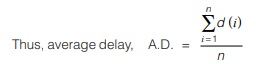

(d) Queue length : It is defined as vertical distance between cumulative arrival and cumulative departure h at any time t. It is represented by q(t) in the figure.

It is to be noted that curve of cumulative arrival continuously increases because arrival of vehicles at intersection does not depend upon whether the traffic signal is red or green although the rate of arrival of vehicle may be different depicted by variable slope of curve of cumulative arrival at different time instants.

<< Previous | Next >>
Must Read: What is Highway Engineering?