Various Types of Thickness of Boundary Layer

(i) Boundary Layer Thickness (Nominal or Normal Thickness) (δ)

• It is defined as the perpendicular distance from the body surface in which velocity reaches 99% of the velocity of the free stream velocity (U∞) i.e. u = 0.99U_∞.

(ii) Displacement Thickness  (δ*)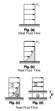

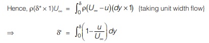
• It is defined as the perpendicular distance by which the boundary surface should be shifted in order to compensate for the reduction in mass flow rate on account of boundary layer formation.

Where, U_∞ = free stream velocity
u = velocity at any distance ‘y’ from body surface

The above formula can be derived as :
If flow is ideal and there is no formation of boundary layer, then the velocity profile would be as shown in Figure (a). But in case of real fluid flow, velocity profile would be as shown in Figure (b)
Here, reduction in mass flow rate is equal to the shaded area. Mass flow rate in 1 will be equal to mass flow rate in 2 or in other words, mass flow rate in 3 is same as that in 4.

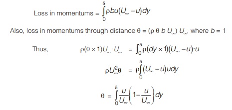
(iii) Momentum Thickness (θ)

It is defined as the perpendicular distance from the boundary surface by which boundary should be shifted in order to compensate for the reduction in momentum of the flowing fluid is due to the boundary layer formation.

Momentum of fluid = mass × flow velocity

= (ρubdy)u

(iv) Energy Thickness (δ_E)

It is defined as the perpendicular distance from the boundary surface such that the energy flux corresponding to the main stream velocity U∞ through the distance δE is equal to the deficiency or loss of energy due to the boundary layer formation.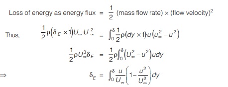

BOUNDARY LAYER SEPARATION

• The boundary layer thickness is considerably affected by pressure gradient in the direction of flow.
• If ∂p/∂x is zero, then the boundary layer continues to grow in thickness along a flat plate.
• With the decreasing pressure as the flow accelerates i.e. with negative (favourable) pressure gradient, the boundary layer tends to be reduced in thickness. It is favourable or desirable because boundary layer in such an accelerating flow is attached closely to the wall and therefore is not likely to separate from the wall.
• With the increasing pressure as the flow declerates i.e. with positive (adverse) pressure gradient, the boundary layer thickens rapidly. This condition is not desirable because if the boundary layer is thicker it does not usually remain attached closely to the wall and is much more likely to separate from the wall.
• The adverse (positive) pressure gradient plus the boundary shear decreases the momentum in the boundary layer.
• If kinetic energy of fluid is not able to overcome the adverse pressure gradient and shear, this results in separation of boundary layers.
• The point on the solid at which the boundary layer is on the verge of separation from the surface is called the point of separation. point of separation
• In turbulent flow, momentum transfer is possible i.e. layer near to body surface may take energy from adjacent layers. In laminar flow no momentum transfer is possible hence laminar boundary layer is more prone to early separation than the turbulent boundary layer.

Buckingham’s π–Method

• This method is used when the variables are more than the number of fundamental dimensions (M,L,T.)
• The theorem states that if there are n dimensional variables (independent and dependent variables) involved in a physical phenomenon, which can be completely described by m fundamental quantities or dimensions (such as mass, length, time etc.), and are related by dimensionally homogeneous equation, then the relationship among the n-quantities can always be expressed in terms of exactly (n – m) dimensionless and independent π terms.
• In a general dimensional analysis problem, there is one π term that we call the dependent π, giving it the notation π. The parameter π, is (in general) a function of several other π′s, which we call independent π′s. Thus, π₁ = f(π₂ , π₃ , . . . . π_k)
  where k is the total number of π′s.
• The method of dimensional analysis of a physical phenomenon involves the following steps :

1. List the parameters or variables (dimensional variables, non dimensional variables and dimensional constants) and count them. Let ‘n’ be the total number of parameters in the problem, including the dependent variable.
2. List the primary dimensions for each of the n parameters. Let ‘m’ be the total number of primary dimensions. Then the expected number of dimensionless π terms will be k = n – m
3. Choose m repeating parameters or variables among them that will be used to construct each π. These variables should be such that none of them is dimensionless and no two variables have the same dimensions.
4. Generate the π′s one at a time by grouping the m repeating parameters with one of the remaining parameters, forcing the product to be dimensionless. In this way, construct all the k π′s.
5. Write the final functional relationship as
   π1 = f(π2, π3, π4 . . . )

Guidelines for Selecting Repeating Variables

The following points should be kept in view while selecting the repeating variables :

• Select the first repeating variable from those describing the geometry of flow e.g. size and shape of fluid passage or of the removing body such as diameter, length, height, etc.
• Select the second repeating variable from those representing the fluid properties such as density, viscosity, surface tension, elasticity, vapour pressure, etc.
• Select the third repeating variable from those characterizing the fluid motion such as velocity, acceleration, discharge, pressure, force, power.

<< Previous | Next >>
Must Read: What is Fluid Mechanics?