Per Capita Demand (Q)

It is the annual average amount of daily water required by one person and includes the domestic use, industrial use and commercial use, public use, waste thefts etc.

It may be, therefore expressed as Per Capita Demand(q) in litres per day per person …(i)

= Total yearly water requirement of the city in litres (i.e V) / 365 × Design Population

Thus, total yearly requirement of city can be estimated using eq. (i) provided that per capita demand is already known or assumed.

For an average Indian city, as per recommendation of I.S. code, the per capita demand(q) may be taken as given in table.

Break up for per capita demand (q) for an average Indian City
Use	Demand in /pcd
(i) Domestic Use (ii) Industrial Use (iii) Commercial Use (iv) Civic or Public Use (v) Waste and thefts, etc. (vi) Fire demand	200 (59.7% or 60%) 50 20 10 55 < 1
	Total = 335         = Per Capita Demand (q)

DESIGN PERIOD OF WATER SUPPLY UNIT

A water supply scheme includes huge and costly structures (such as dams, reservoirs, treatment works, penstock pipes, etc.) which cannot be replaced or increased in their capacities, easily and conveniently. For example, the water mains including the distributing pipes are laid underground, and cannot be replaced or added easily, without digging the roads or disrupting the traffic. In order to avoid these future complications of expansion, the various components of a water supply scheme are purposely made larger, so as to satisfy the community needs for a reasonable number of years to come. This future period or the number of years for which a provision is made in designing the capacities of the various components of the water supply scheme is known as design period. design period The design period should neither be too long nor should it be too short.

Factors Governing the Design Period

The design period cannot exceed the useful life of the component structure, and is guided by the following considerations:

1. Useful life of component structures and the chances of their becoming old and obsolete. Design period should not exceed their respective values.
2. Ease and difficulty that is likely to be faced in expansions, if undertaken at future dates.
3. Amount and availability of additional investment likely to be incurred for additional provision.
4. The rate of interest on the borrowings and the additional money invested.
5. Anticipated rate of population growth, including possible shifts in communities, industries and commercial establishment.

Design Period Values

Water supply projects, under normal circumstances, may be designed for a design period of 30 years excluding completion time of 2 years. The design period recommended by the GOI manual on water supply for designing the various components of a water supply projects are given below:

 

Design periods for components of a water supply scheme
S.No.	Item	Design period in years
1. 2. 3. 4. 5. 6. 7. 8.	Storage by dams Intake works Pumping (i)  Pump house (ii) Electric motors and pumps Water treatment units Pipe connections to the several treatment units and other small appurtenances Raw water and clear water conveying units Clear water reservoirs at the head works, balancing tanks, and Services reservoirs (over-head or ground level) Distribution system	50 30 30 15 15 30 30 15 15 30

Population Forecasting Methods

The various methods which are generally adopted for estimating future populations by engineers are described in this section. Some of these methods are used when design period is small, and some are used when the design period is large. The particular method to be adopted for a particular case or for a particular city depends largely upon the factor discussed in these methods and the selection is left to the discretion and intelligence of the designer. It is to be noted that none of these methods is exact and all the methods are based on law of probability.

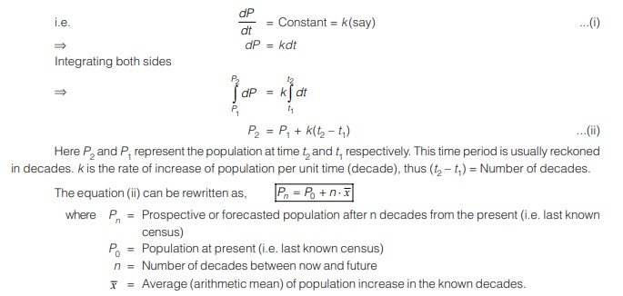
(a) Arithmetic Increase Method

In this method, a constant increment of growth in population is observed periodically. This method is of limited application, mostly used in large and established towns where future growth has been controlled. This method is based upon the assumption that the population increase at a constant rate, i.e. the rate of change of population with time (dP / dt) is constant.

(b) Geometric Increase Method

The method of Geometric progression is applicable to the cities with unlimited scope for future expansion and where a constant rate of growth is anticipated. This method is also known as uniform increase method. uniform increase method.
The basic difference between arithmetic and geometric progression or increase method of population forecasting is that, in Arithmetic method no compounding is done whereas, in Geometric method compounding is done every decade. To have better understanding of difference between arithmetic increase method and geometric increase method, consider a city having population of 1 lakh.

If the growth rate of population is 10% per decade, then at end of first decade from now, population will be 1.1 lakhs by both the methods. But at the end of 2nd decade, population will be 1.21 lakh by geometric increase method whereas it will be 1.2 lakh only by arithmetic increase method. The computations in these two methods i.e. arithmetic and geometric increase are thus comparable to simple and compound interest computations respectively.

In Geometric increase method, a constant value of percentage growth rate per decade (k) is analogues to the rate of compounding interest per annual.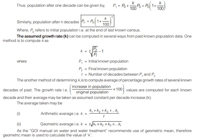

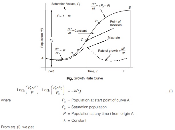
(i) The Logistic curve method

Consider again the population growth curve that is discussed earlier. It is assumed that under normal conditions, the population of a city shall grow as per the logistic curve, shown in figure. As per P.F. verhulst, the entire curve AE can be represented by an autocatalytic first order reaction given as

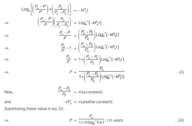
Equation (iii) it is the required equation of logistic curve. McLeau suggested that if only three pair of population values P₀, P₁ and P₂ at times t = 0, t = t₁ and t = 2t₁ extending over the useful range of census populations are chosen, the constant m and n and saturation population P_s can be determined as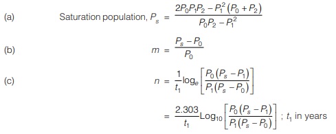

<< Previous | Next >>
Must Read: What is Environmental Engineering?